Skip to main content

Demographic Transition in Brazil

Theoretical foundations and historical evidence

Visual and data companion for the chapter by Turra and Fernandes (2026).

Authors

Affiliations

Cassio M. Turra

Centro de Desenvolvimento e Planejamento Regional (Cedeplar), Universidade Federal de Minas Gerais (UFMG)

Fernando Fernandes

Independent Researcher

de·mo·graph·ic tran·si·tion en-US /ˌdɛməˈɡræfɪk trænˈzɪʃən/ noun A long-run shift from high to low mortality and fertility levels, changing population age structure and demographic dependency patterns.

About

This page accompanies the chapter:

Turra, Cassio M.; Fernandes, Fernando. A transição demográfica no Brasil: fundamentos teóricos e evidências históricas. In: Martins, Richarlls; Miranda-Ribeiro, Paula (eds.). Populações e desenvolvimento: 30 anos pensando, repensando e construindo o Brasil. Rio de Janeiro, RJ: Círculo de Giz, 2026, p. 115-153. ISBN 978-65-997182-9-8.

In roughly 80 years — from the 1940s to the 2020s — Brazil completed a demographic shift that took European pioneer societies two centuries. Infant mortality fell from roughly 150 per 1,000 live births in 1940 to around 30 by the early 2000s; total fertility dropped from more than six children per woman in the 1960s to approximately 1.6 today, well below replacement level. The dataset provides annual population growth rates, child and old-age dependency ratios, and demographic dividend estimates for Brazil and all federative units across historical census benchmarks (1872–2000, including the 1991–2000 bridge period) and annual population projections through 2070. This companion highlights population growth by period and the full indicator table; the chapter on ResearchGate includes all four figures from the book.

Figures

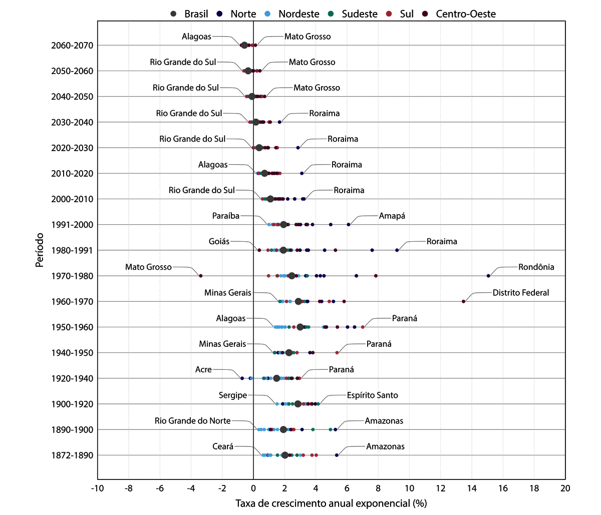
Population growth by period

Population growth: average annual rate by period, Brazil and federative units, 1872–2070.

Data

The demographic indicators are available in the interactive table below. Use the filters to select the geographic level, unit, period type, and — for the projection segment (2000–2070) — the resolution (5-year or 1-year); historical periods (1872–2000) are fixed census benchmarks at every resolution. You can also download the full dataset (CSV) — the file includes citation and license metadata as commented header lines (#).

Filters. Geographic level selects Brazil (national), Regions, or States. Unit narrows to a specific region or state when the level allows. Period selects all periods, historical census benchmarks (1872–2000), or annual projections (2000–2070).

Data limitations. Census population counts were not historically reconciled or evaluated for geographical coverage, completeness, or common data problems. Although the series may be adjusted in specific studies, such adjustments would not alter the chapter’s conclusions about major trends.

Geographic level

Unit

Period

Resolution

Download filtered CSV

Rows per page

Visual Trends

Time series for the selected geography, from the first census benchmark (1872) through 2070 projections. The dashed vertical line marks the 2000 boundary between census data and IBGE estimates and projections.

csvRaw = FileAttachment("assets/data/dtb-indicators-1872-2070.csv").text()

// Figures always plot the projection segment (2000-2070) at 1-year (annual)
// resolution, independent of the companion table's Resolution filter — the
// CSV's `granularity` column tags historical census rows as "historical"
// (always kept) and projection rows as "5-year" or "1-year" (only "1-year"
// kept here).
allRows = {
  const clean = csvRaw
    .split("\n")
    .filter(l => l.trim() && !l.trimStart().startsWith("#"))
    .join("\n")
  return d3.csvParse(clean, r => ({
    geo_level:   r.geo_level,
    geo_sigla:   r.geo_sigla,
    geo_name_en: r.geo_name_en,
    period:      r.period,
    granularity: r.granularity,
    year_start:  +r.period.split("-")[0],
    year_end:    +r.period.split("-").at(-1),
    pop_start:   +r.pop_start / 1e6,
    pop_end:     +r.pop_end   / 1e6,
    growth_r:    +r.growth_r_pct,
    cadr:        +r.cadr_pct,
    oadr:        +r.oadr_pct,
    dividend:    +r.demo_dividend_pct
  })).filter(r => r.granularity === "historical" || r.granularity === "1-year")
}

T = ({
  young:    "#6a9bcc",
  old:      "#b5654a",
  div:      "#5e7245",
  dividend: "#8c1d40",
  bg:       "#F9F8F6",
  ink:      "#242424",
  grey:     "#525252",
  border:   "#dedad3"
})
// Mirrors $font-family-monospace (caro-tokens.scss): keeps SVG labels identical
// to the .dtb-strip-header HTML font. Update both if the canonical mono stack changes.
MONO  = "Spline Sans Mono, SFMono-Regular, Consolas, 'Liberation Mono', monospace"
X_DOM = [1866, 2078]
X_TKS = [1875, 1900, 1925, 1950, 1975, 2000, 2025, 2050, 2075]
PROJ  = 2000

viewof geoLevel = Inputs.radio(["Country", "Region", "State"], {
  value: "Country",
  label: "Geographic level"
})

geoIbgeOrder = JSON.parse(document.getElementById("dtb-geo-ibge-order").textContent)

// Same citation/license/page lines as get_companion_csv_header() (R), reused
// verbatim in the downloaded PNG footer so the two never drift apart.
citationLines = JSON.parse(document.getElementById("dtb-citation-lines").textContent)

levelUnits = {
  const lvl = geoLevel.toLowerCase()
  const seen = new Set()
  const units = allRows.filter(r => {
    if (r.geo_level !== lvl || seen.has(r.geo_sigla)) return false
    seen.add(r.geo_sigla)
    return true
  })
  const order = geoIbgeOrder[lvl] || []
  const rank = new Map(order.map((sigla, i) => [sigla, i]))
  return units.sort((a, b) => {
    const ai = rank.has(a.geo_sigla) ? rank.get(a.geo_sigla) : 999
    const bi = rank.has(b.geo_sigla) ? rank.get(b.geo_sigla) : 999
    return ai - bi
  })
}

viewof geoUnit = Inputs.select(levelUnits, {
  label: "Unit",
  format: d => d.geo_name_en
})

rows = allRows
  .filter(r => r.geo_level === geoUnit.geo_level && r.geo_sigla === geoUnit.geo_sigla)
  .sort((a, b) => a.year_start - b.year_start)

mkSeries = key => rows.map(r => ({x: r.year_start, y: r[key]}))
popLine = rows.length ? [
  ...rows.map(r => ({x: r.year_start, y: r.pop_start})),
  {x: rows.at(-1).year_end, y: rows.at(-1).pop_end}
] : []

// One PNG for the whole stack: the panel SVGs (titles already inside them) drawn
// top-to-bottom onto a single 2× canvas — what you see on the page is what is saved.
function dlStack(charts, name) {
  const scale = 2, gap = 8
  const dims = charts.map(c => c.getBoundingClientRect())
  const w = dims[0].width
  const totalH = dims.reduce((a, d) => a + d.height + gap, 0)
  const canvas = Object.assign(document.createElement("canvas"), {
    width: Math.round(w * scale), height: Math.round(totalH * scale)
  })
  const ctx = canvas.getContext("2d")
  ctx.scale(scale, scale)
  ctx.fillStyle = T.bg
  ctx.fillRect(0, 0, w, totalH)

  const loads = charts.map((c, i) => new Promise(resolve => {
    const blob = new Blob([new XMLSerializer().serializeToString(c)],
      {type: "image/svg+xml;charset=utf-8"})
    const url = URL.createObjectURL(blob)
    const img = new Image()
    img.onload = () => { URL.revokeObjectURL(url); resolve({img, h: dims[i].height}) }
    img.src = url
  }))

  Promise.all(loads).then(parts => {
    let y = 0
    for (const p of parts) { ctx.drawImage(p.img, 0, y); y += p.h + gap }
    Object.assign(document.createElement("a"),
      {download: name, href: canvas.toDataURL("image/png")}).click()
  })
}

// Single strip-panel chart (Observable Plot SVG). The title + subtitle are drawn
// as SVG <text> in the top margin (not HTML), so the on-page panel and the exported
// PNG are the same artifact. Subtitle dx uses the Source Code Pro monospace advance
// (~0.6em) — same trick as Demographic Flux's drawStripPanelChrome.
// fontFamily/color must be top-level — Plot ignores `style` inside x/y scales,
// so axis ticks would otherwise fall back to the default sans instead of MONO.
// Geometry mirrors Demographic Flux viewer constants (flux-layout.js / flux-panels.js):
//   PAD_L = 74 → marginLeft
//   title at top − 12 → dy: −12 on both title and subtitle text marks
//   subtitle x = PAD_L + title.length * 8.4 + 14 → dx: title.length * 8.4 + 14
//   "calendar year" centred below bottom axis (drawPeriodAxis) → manual text mark, no Plot label
// These are the only canonical strip-panel geometry constants; there is no separate
// caro-quarto spec document — flux-layout.js / flux-panels.js are the source of truth.
buildChart = ({title, sub, marks, yZero = false, xLabels = false}) => Plot.plot({
  width,
  height: xLabels ? 186 : 162,
  marginLeft: 74, marginRight: 88,
  marginTop: 28, marginBottom: xLabels ? 44 : 10,
  style: {background: T.bg, overflow: "visible", fontFamily: MONO, fontSize: "11px", color: T.grey},
  x: {
    domain: X_DOM, ticks: X_TKS, grid: true,
    label: null,
    tickFormat: xLabels ? d => String(d) : () => "",
    tickSize: xLabels ? 5 : 2
  },
  y: {label: null, nice: true, zero: yZero},
  marks: [
    Plot.text([title.toUpperCase()], {
      frameAnchor: "top-left", textAnchor: "start", dy: -12,
      text: d => d, fontSize: 13, fontFamily: MONO, fill: T.ink
    }),
    Plot.text([sub], {
      frameAnchor: "top-left", textAnchor: "start",
      dx: title.length * 8.4 + 14, dy: -12,
      text: d => d, fontSize: 11, fontFamily: MONO, fill: T.grey
    }),
    ...(xLabels ? [Plot.text(["calendar year"], {
      frameAnchor: "bottom", dy: 38,
      text: d => d, fontSize: 12, fontFamily: MONO, fill: T.ink
    })] : []),
    Plot.ruleX([PROJ], {stroke: T.grey, strokeDasharray: "3,3", strokeWidth: 1, strokeOpacity: 0.7}),
    ...marks
  ]
})

wrapMono = (text, maxChars) => {
  const words = text.split(" ")
  const lines = []
  let line = ""
  for (const w of words) {
    const candidate = line ? line + " " + w : w
    if (candidate.length > maxChars && line) {
      lines.push(line)
      line = w
    } else {
      line = candidate
    }
  }
  if (line) lines.push(line)
  return lines.join("\n")
}

buildHeaderPanel = label => Plot.plot({
  width,
  height: 30,
  marginLeft: 74, marginRight: 88, marginTop: 0, marginBottom: 0,
  style: {background: T.bg, overflow: "visible", fontFamily: MONO, fontSize: "11px", color: T.ink},
  marks: [
    Plot.text([label.toUpperCase() + "\u00a0\u00b7\u00a0DEMOGRAPHIC INDICATORS, 1872\u20132070"], {
      frameAnchor: "left", textAnchor: "start",
      text: d => d, fontSize: 14, fontFamily: MONO, fontWeight: 700, fill: T.ink
    })
  ]
})

buildFooterPanel = lines => {
  const innerWidth = width - 74 - 88
  const fontSize = 9.5
  const maxChars = Math.max(40, Math.floor(innerWidth / (fontSize * 0.62)))
  const text = lines.map(l => wrapMono(l, maxChars)).join("\n")
  const lineCount = text.split("\n").length
  return Plot.plot({
    width,
    height: lineCount * 13 + 12,
    marginLeft: 74, marginRight: 88, marginTop: 6, marginBottom: 6,
    style: {background: T.bg, overflow: "visible", fontFamily: MONO, fontSize: fontSize + "px", color: T.grey},
    marks: [
      Plot.text([text], {
        frameAnchor: "top-left", textAnchor: "start", lineAnchor: "top",
        text: d => d, fontSize, fontFamily: MONO, fill: T.grey, lineHeight: 1.35
      })
    ]
  })
}

fmtSigned = (v, digits, unit) => (v >= 0 ? "+" : "") + v.toFixed(digits) + unit

// dot + end label on the final datum (dx/dy mirror Demographic Flux drawEndLabel:
// dot radius 2.5, label offset dx 8 / dy -5). dy is overridable to de-conflict.
endMarks = (data, color, fmt, dy = -5) => {
  const last = data.slice(-1)
  return [
    Plot.dot(last, {x: "x", y: "y", fill: color, r: 2.5}),
    Plot.text(last, {
      x: "x", y: "y", dx: 8, dy, textAnchor: "start",
      text: d => fmt(d.y), fill: color, fontSize: 11, fontFamily: MONO
    })
  ]
}

// full line series: stroke + end marker. strokeOpacity 0.9 mirrors Demographic
// Flux's line alpha (230/255) — full saturation reads too vivid against the cream.
lineMarks = (data, color, fmt, dy = -5) => [
  Plot.line(data, {x: "x", y: "y", stroke: color, strokeWidth: 1.6, strokeOpacity: 0.9}),
  ...endMarks(data, color, fmt, dy)
]

// Whole figure stack: four strip panels (header + chart) in one container, with a
// single ↓ PNG button that exports the entire stack as one composite image.
trendsStack = {
  const specs = [
    {title: "Population", sub: "millions \u00b7 beginning of period",
     marks: lineMarks(popLine, T.young, v => v.toFixed(1) + "\u00a0M")},
    {title: "Crude Growth Rate", sub: "mean annual \u00b7 % per year", yZero: true,
     marks: [Plot.ruleY([0], {stroke: T.border, strokeWidth: 0.9}),
             ...lineMarks(mkSeries("growth_r"), T.div, v => fmtSigned(v, 2, "%\u00a0/\u00a0yr"))]},
    {title: "Dependency Ratios",
     sub: "child/adolescent and old-age \u00b7 % of working-age (20\u201364)",
     marks: [...lineMarks(mkSeries("cadr"), T.young, v => "CADR\u00a0" + v.toFixed(1) + "%", 16),
             ...lineMarks(mkSeries("oadr"), T.old,   v => "OADR\u00a0" + v.toFixed(1) + "%", -18)]},
    {title: "Demographic Dividend", sub: "annual \u00b7 % per year", yZero: true, xLabels: true,
     marks: [Plot.ruleY([0], {stroke: T.border, strokeWidth: 0.9}),
             ...lineMarks(mkSeries("dividend"), T.dividend, v => fmtSigned(v, 2, "%\u00a0/\u00a0yr"))]}
  ]

  const stack = document.createElement("div")

  function appendPanel(panel) {
    const wrap = document.createElement("div")
    wrap.className = "dtb-strip-chart"
    wrap.append(panel)
    stack.append(wrap)
    return panel
  }

  // Header (geo unit) and footer (citation) travel with the on-page view and
  // the downloaded PNG alike — both are plain SVG panels in `charts`.
  const charts = [
    appendPanel(buildHeaderPanel(geoUnit.geo_name_en)),
    ...specs.map(s => appendPanel(buildChart(s))),
    appendPanel(buildFooterPanel(citationLines))
  ]

  const btn = Object.assign(document.createElement("button"), {
    className: "dtb-download-btn", textContent: "\u2193\u00a0PNG"
  })
  btn.onclick = () => dlStack(charts, `dtb-visual-trends-${geoUnit.geo_sigla.toLowerCase()}.png`)
  stack.append(btn)
  return stack
}

Variables

Notation	CSV column	Description
Geographic unit	geo_name_en	Region or state name in English, matching the page language (national level shows Brazil)
Period	period	Period label (e.g. 1872–1890 for historical benchmarks; 5-year or 1-year labels for projections, depending on the Resolution filter)
N0	pop_start	Total population at the beginning of the period (both sexes)
N1	pop_end	Total population at the end of the period (both sexes)
r	growth_r_pct	Mean annual exponential growth rate (% p.a.)
CADR	cadr_pct	Child/adolescent dependency ratio (%): population aged 0–19 relative to 20–64
OADR	oadr_pct	Old-age dependency ratio (%): population aged 65+ relative to 20–64
Dividend	demo_dividend_pct	Annual demographic dividend (% p.a.) from dependency-ratio change

Notation: dependency ratios and growth follow the chapter definitions (Turra & Fernandes 2026). Filter-only columns (geo_level, geo_sigla, geo_name_pt, granularity) remain in the downloadable CSV but are not shown in the table. granularity (historical | 5-year | 1-year) backs the Resolution filter, which controls the projection segment's (2000–2070) resolution in the table; historical rows (census benchmarks) appear regardless of the selected resolution, and the Visual Trends figures below always use 1-year data for the projection segment.

Sources

IBGE. 1956. VI Recenseamento Geral Do Brasil - 1950: Censo Demográfico (Resultados Finais). Série Nacional e Regional. IBGE, Serviço Nacional de Recenseamento.

IBGE. 1962–1966. VII Recenseamento Geral Do Brasil - 1960: Censo Demográfico (Resultados Finais). Série Nacional e Regional. IBGE, Serviço Nacional de Recenseamento.

IBGE. 1973. Censo Demográfico 1970: Resultados Finais (Brasil e Unidades Da Federação). Série Nacional e Regional. Instituto Brasileiro de Geografia e Estatística.

IBGE. 1982. Censo Demográfico 1980: Resultados Finais (Brasil e Unidades Da Federação). Série Nacional e Regional. Instituto Brasileiro de Geografia e Estatística.

IBGE. 1994. Censo Demográfico 1991: Resultados Do Universo (Brasil e Unidades Da Federação). Instituto Brasileiro de Geografia e Estatística.

IBGE. 2024. Projeções da população: Brasil e unidades da federação - revisão 2024. Notas metodológicas, 01/2024. IBGE, Coordenação de População e Indicadores Sociais.

Questions

For problems or questions, please open an issue.

License

This site is licensed under CC BY-NC 4.0.